Distribution in the Wyckoff model is an inferred reduction of holdings, often after an advance. Candlesticks cannot identify buyers and sellers; observable evidence remains price, time and available volume.
Establishing the range
BC, buying climax, describes climactic buying; AR, automatic reaction, the subsequent decline; ST, secondary test, revisits the high area. They help outline resistance and support.
An advance can also stop without an obvious climax. Compare new reactions with earlier ones: progress, speed of return and accompanying volume.
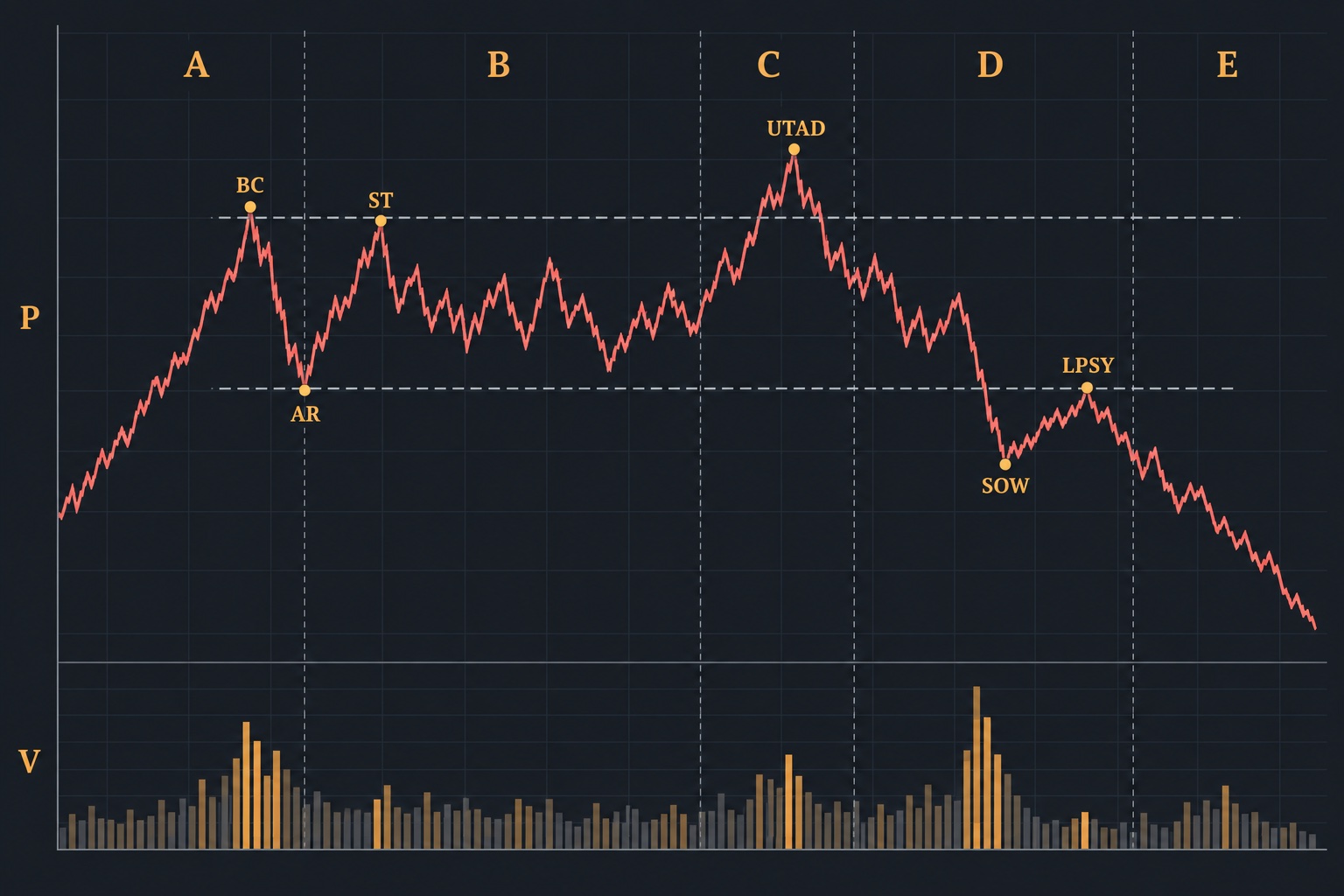
Hypothetical sequence
Price advances from 80 to 110, reacts to 100, then returns toward 108–110. A later move to 112 returns inside the range. In an appropriate context it is an upthrust or late UTAD candidate.
A subsequent decline through 100 and a weak recovery near 100–101 are compatible with SOW and LPSY. These illustrative prices do not set a trade target.
Counterexample: reaccumulation
A range after an advance may lead to another advance. Sustained price above resistance requires reconsidering the distribution hypothesis; do not retain a label against new evidence.
UTAD is not mandatory. Not every new high is UTAD: its place in the developing structure and subsequent behaviour matter.
Keep observations separate
Distinguish the range, boundary penetration, return and later holding behaviour. Volume must be comparable in source and units. A strong news bar does not prove a completed schematic.
See Bruce Fraser’s Distribution Definitions. Continue with SOW and LPSY.